Basic Probability

Statistical hypothesis testing involves estimating the probability of obtaining a particular result, e.g. the sample mean, or something more extreme, if the null hypothesis were true. If the probability of getting the result is low, i.e., below a certain threshold, you conclude that the null hypothesis is probably not true. So, let’s familiarize ourselves with some basic probability.

Notation

We will define an event as \(E\). For example, \(E\) could be getting tails when you flip a coin or getting a 2 when you roll a die.

We define the probability of \(E\) as \(Pr(E)\).

For the example of getting a 2 when you roll a die,

\[ Pr(E) = \frac{1}{6} \]

The probability of \(E\) not happening is defined as,

\[ Pr(\tilde{E}) = 1 - Pr(E) \]

For the example of rolling the die,

\[\begin{split} \begin{align} Pr(\tilde{E}) & = 1 - \frac{1}{6}\\ & = \frac{5}{6} \end{align} \end{split}\]

Unions and Intersections

The probability that two events, \(E_1\) (rolling a 5) and \(E_2\) (rolling a 6) will both occur is called the intersection of the two probabilities and is denoted as

\[ Pr(E_1 \cap E_2) \]

This is sometimes also called the joint probability of \(E_1\) and \(E_2\).

The probability that either or both of the two events, \(E_1\) (rolling a 5) and \(E_2\) (rolling a 6) will occur is called the union of the two probabilities. This is denoted as

\[ Pr(E_1 \cup E_2) = Pr(E_1) + Pr(E_2) - Pr(E_1 \cap E_2) \]

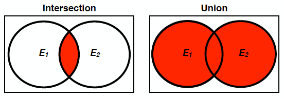
Fig. 6 Venn diagram of an intersection and a union of events \(E_1\) and \(E_2\).

Figure Fig. 6 shows a Venn diagram visualization of the meaning of intersection and union of events \(E_1\) and \(E_2\). Notice visually how the probability of the union is equal to the sum of the two individual probabilities minus the probability of the intersection - we do not want to double count the region where the two individual probabilities intersect.

Conditional probability

The final concept we will discuss is conditional probability. The conditional probability of the event \(E_2\) is the probability that the event will occur given the knowledge that a particular event, for example, \(E_1\), has already occurred. We denote this conditional probability as follows:

\[ Pr(E_2|E_1) \]

and we typically say “the probability of \(E_2\) given \(E_1\)”.

The above conditional probability is defined as

\[ Pr(E_2|E_1) = \frac{Pr(E_1 \cap E_2)}{Pr(E_1)} \]

Rearranging this conditional probability formula yields the probability of the intersection, called the multiplicative law of probability:

\[ Pr(E_1 \cap E_2) = Pr(E_2|E_1) \cdot Pr(E_1) = Pr(E_1|E_2) \cdot Pr(E_2) \]

If \(E_1\) and \(E_2\) are independent events, i.e. their probabilities do not depend on each other, then the conditional probability is simply,

\[ Pr(E_2|E_1) = Pr(E_2) \]

and consequently,

\[ Pr(E_1 \cap E_2) = Pr(E_2) \cdot Pr(E_1) \]

This is the formal definition of statistical independence for two events.

Note

Two events \(E_1\) and \(E_2\) are independent if and only if their joint probability equals the product of their probabilities.

For example, rolling a fair die yields statistically independent events. Therefore, the joint probability of rolling both a 5 (\(E_1\)) and a 6 (\(E_2\)) is equal to

\[\begin{split} \begin{align} Pr(E_1 \cap E_2) & = Pr(E_2) \cdot Pr(E_1)\\ & = \frac{1}{6} \cdot \frac{1}{6}\\ & = \frac{1}{36} \end{align} \end{split}\]

###ADD interactive buttons here###