
Estimating Statistical Significance with a z-test#
So, how do we test whether the mean of the sample is different from the mean of the population? We can use the \(z\)-statistic!
Again, recall that the \(z\)-statistic is defined as,
where \(\mu\) is the population mean and \(\sigma\) is the population standard deviation and \(x\) is normally distributed.
Now, we want to assess the probability of \(\overline{x}\), not \(x\). So, we replace \(\mu\) with the population mean of the \(\overline{x}\) and \(\sigma\) with the population standard deviation of \(\overline{x}\).
Note that,
Plugging these in leads to,
The \(z\)-statistic is now the number of standard errors that the sample mean deviates from the population mean.
We can easily manipulate the above equation for the \(z\)-statistic to obtain an equation for the difference of two means, \(x_1\) and \(x_2\) (as opposed to the difference between a sample mean and the population), where \(\sigma_1\) can be different from \(\sigma_2\):
\(\Delta_{1,2}\) is the null hypothesized difference between the two means, which is typically zero in practice.
Let’s revisit our ENSO example to apply the above to real data. First, we will look at an example using the \(z\)-statistic for a single value of our ENSO index and then we will look at an example using the \(z\)-statistic for a sample of our ENSO index.
Question #1
What is the probability that December 2013 had an ENSO index of -0.50 or less? Assume that the ENSO index is standard normal.
To answer this, we will simply use our \(z\)-table as we did two sections ago.
import scipy.stats as st
import numpy as np

#Question #1
p = st.norm.cdf(-0.5)
print(round(p,4))
0.3085
Thus, there is a ~31% likelihood that the December 2013 ENSO index could have a value of -0.5 or less.
Question #2
What is the probability that the average 2003-2013 monthly ENSO index was -0.50 or less (assuming that ENSO dynamics have not changed)? Assume that the ENSO index is standard normal.
Before we answer this, let’s reframe the question in terms of a null and alternative hypothesis. What is our null hypothesis? In this case our null hypothesis would be that the sample mean ENSO index of -0.5 is the same as the population mean, which is zero in this case (ENSO is standard normal). The alternative hypothesis is that the sample mean and population mean are different.
We will use the \(z\)-statistic to answer this question, in other words, we will perform a z-test.
First, how big is our sample? We have a sample of ENSO indices which is 10 years x 12 months per year in size, giving \(N\) = 120.
Next, let’s write down what we know:
Plugging these into our \(z\)-statistic equation, we get
We can now look up this value for \(z\) in our \(z\)-table.
#Question #2
p = st.norm.cdf(-5.48)
print(p)
2.126629179795902e-08
This is a very small value, indicating that this is a very rare event. We can conclude that the sample mean ENSO index for 2003-2013 is different from the population mean.
In statistical hypothesis testing, we typically use a threshold probability for which we reject the null hypothesis. The threshold is often 5%, e.g. if there is less than a 5% chance that the sample mean and the population mean are the same, then we reject the null hypothesis and we say “the sample mean is significantly different from the population mean”
Hypothesis Testing Revisited#
Terminology#
Let’s formalize the steps we went through above to perform a \(z\)-test with some terminology:
significance/confidence level: the significance level, \(\alpha\), is the threshold and is typically 5% (0.05). This is often reported as the confidence level, 1 - \(\alpha\), e.g. “the 95% confidence level”.
critical value: \(z_c\), the value of \(z\) that must be exceeded to reject the null hypothesis. The value of \(z_c\) depends on the formulation of your alternative hypothesis, i.e. is a one-sided \(z_{\alpha}\), two-sided \(z_{\alpha/2}\) test appropriate (more on this below).
p-value: the probability of observing a signal given that the null hypothesis is true (probability of your \(z\)-statistic).
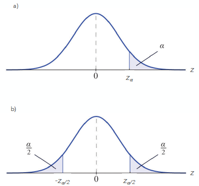
Fig. 9 The area under the curve for a (a) one-sided and (b) two-sided \(z\)-test.#
Note
Figure 9 depicts the critical value, \(z_c\) and the significance level, \(\alpha\), for a one-sided and two-sided \(z\)-test. In practice, you will almost always perform a two-sided test. This means that we are testing whether there is a signal but we do not know the sign of the signal, e.g. the alternative hypothesis is that the sample mean is different from the population mean, but we don’t know whether it’s greater than or less than the population mean. This is a more conservative test. In specific cases, a one-sided test may be appropriate (follow this link to learn more).
Five Simple Steps#
In using statistical significance tests, there are 5 simple steps that should be followed, in order.
State the significance level (\(\alpha\))
State the null hypothesis \(H_0\) and the alternative \(H_1\)
State the statistic to be used\(^*\), and the assumptions required to use it
State the critical region (one-sided or two-sided test)
Evaluate the statistic and state the conclusion
\(^*\)for now we are just using the \(z\)-statistic.
Let’s go through an example following these 5 steps.
Question #3
Sam is a ski instructor and went skiing 60 times at Mont Tremblant this winter. The average temperature on these 60 days was -7°C, and the standard deviation of 60 daily temperatures is 6°C. Sam knows that the climatological mean winter temperature for Mont Tremblant is -10°C. Is this a sign of climate change?
Try to go through the steps on your own before you take a look at the answers.
Step 1. let’s use the 95% significance level (\(\alpha\) = 0.05)
Step 2. \(H_0\): \(\mu\) = -10°C and \(H_1\): \(\mu\) \(\neq\) -10°C
Step 3. Since we have \(N\) = 60 samples to estimate the true standard deviation (\(\sigma\)) from the sample standard deviation (\(s\)), we can use a \(z\)-test (\(N\) is sufficiently large).
Step 4. We will use a two-sided \(z\)-test (before he went skiing, Sam didn’t know what to expect from the temperatures). Thus, to reject the null hypothesis we must have \(z\) > \(z_{0.025}\) = 1.96.
Step 5. (see code below). Since \(z\) is greater than 1.96, we can reject the null hypothesis and accept the alternative hypothesis that the sample is significantly different from climatology for the days Sam went skiing. Further analysis needs to be done to attribute this to climate change.
Show code cell source
# 5. Now, we compute the z-statistic

z = (-7 + 10)/(6/(np.sqrt(60)))
print(z)
Show code cell output
3.8729833462074166
Errors in Hypothesis Testing#
You may be familiar with the terms “false positive” and “false negative”, but you may not realize that these are statistical terms and are used to categorize possible errors in statistical tests.
For example, when you reject a null hypothesis, there is a chance that you are making a mistake. The null hypothesis might in fact be true, and it may be that your data deviate from the null hypothesis purely by chance. This is an example of a false positive. A false positive (also called a Type I error) occurs when the null hypothesis \(H_0\) is in fact true, but we reject it based on our data. A false negative (also called a Type II error) occurs when the null hypothesis \(H_0\) is in fact false, but we do not reject it based on our test.
Figure 10 illustrates the matrix of possible outcomes of statistical tests. Although it is not possible to know if, for example, your rejection of your null hypothesis is in error, it is important to keep this matrix in mind. This matrix also illustrates why we can never say that a statistical test “proves” our hypothesis; there’s always a small chance that our data are anomalous and differ from the null hypothesis purely by chance.
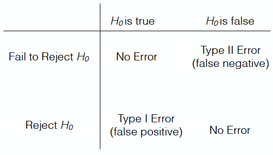
Fig. 10 Matrix of possible outcomes of statistical tests. The rows indicate the outcome of the test and the columns indicate the truth.#
Confidence Intervals#
We can also use the \(z\)-statistic to determine confidence intervals on the true population mean, \(\mu\). Here is an example:
Question #4
Say we have surface air temperatures for 30 winters with a mean of 10°C and a standard deviation of 5°C. What is the 95% confidence interval on the true population mean? You may assume that the temperatures are normally distributed.
In this question, we are told to estimate the 95% confidence intervals. This means we should consider the 95% confidence level, i.e. the 5% significance level.
To estimate the 95% confidence intervals on \(\mu\), we can simply rearrange the equation for \(z\) as follows,
Since we are interested in the 95% confidence intervals centred on \(\mu\), and since the normal distribution is symmetric about the \(\mu\), this can be rewritten as,
where \(z_{\alpha/2}\) is the value for \(z\) for a two-sided 95% confidence level (5% significance level). We can use python get find this value:
# Question #4
# find z values for a two-sided 95% confidence level
zneg = st.norm.ppf(0.025) # negative side of distribution
zpos = st.norm.ppf(0.975) # positive side of distribution
print(round(zneg,2),round(zpos,2))
-1.96 1.96
Plugging this all in, we get
Thus, the 95% confidence intervals on the true population mean, \(\mu\) are,