Non-parametric Correlations

In this section, we will discuss two alternative expressions for correlation that do not depend on any assumptions of normality (aka non-parametric).

Spearman’s Rank Correlation

Spearman’s Rank Correlation is a non-parametric statistic that tests whether a set of paired data monotonically vary together, but it does not assume that the data co-vary linearly. Figure 16 illustrates data that co-vary montonically but not linearly and are perfectly correlated using the Spearman’s Rank Correlation.

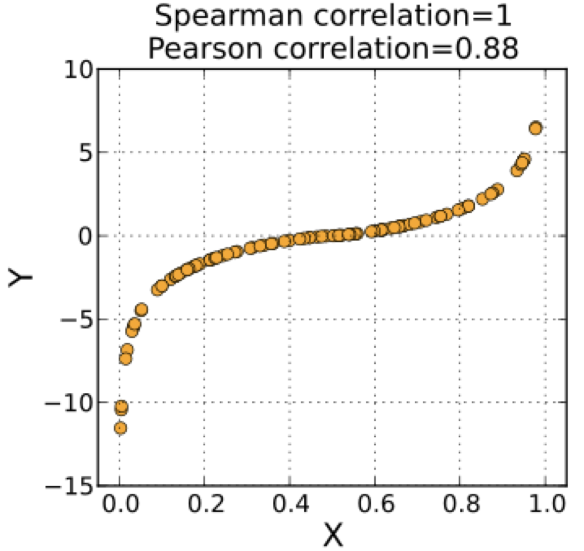
Fig. 16 Scatter plot showing perfectly monotonically co-varying data ref.

The idea is very simple, your original paired data \(x_i\) and \(y_i\) get converted into ranks \(X_i\) and \(Y_i\) from lowest to highest. We then compute the correlation coefficient in the same way as before but using the ranks.

\[ \begin{align} r_{\text{spearman}} = \frac{\overline{X^{\prime}Y^{\prime}}}{\sigma_X\sigma_Y} \end{align} \]

Statistical significance testing for Spearman’s Rank Correlation can be performed using the Fisher-Z transformation.

Let’s compare the Pearson Correlation with the Spearman’s Rank Correlation for our ENSO and California Precipitation Data.

First, we need to load the data.

# load packages
import numpy as np
import pickle as pickle
import scipy.stats as st
import matplotlib.pyplot as plt
import matplotlib as mpl
mpl.rc('font',size=16,weight='bold') #set default font size and weight for plots

# ENSO Data:
# unpickle NINO34 (units of degC)
with open('NINO34_NDJF.pickle','rb') as fp: #.pickle files are a python file type
    nino34 = pickle.load(fp,encoding='latin1')[0]

#  Precipitation Data:
#  unpickle CA_PRECIP_DJFM (units of mm/day)
with open('CA_PRECIP_DJFM.pickle','rb') as fp: #.pickle files are a python file type
    precip_djfm = pickle.load(fp,encoding='latin1')

Let’s remind ourselves of the Pearson correlation between these two variables.

# Pearson's correlation coefficient function including the p-value
pearsons_corrcoef, p_corr = st.pearsonr(nino34,precip_djfm)
print("The Pearson Correlation =",np.round(pearsons_corrcoef,2), "with a very small p-value of", p_corr, "i.e., a very significant correlation!")

The Pearson Correlation = 0.5 with a very small p-value of 2.6350145043512816e-71 i.e., a very significant correlation!

Now let’s take a look at Spearman’s Rank Correlation.

# Spearman's Rank correlation coefficient function including the p-value
spearmans_corrcoef, p_corr = st.spearmanr(nino34,precip_djfm)
print("The Spearman's Rank Correlation =",np.round(spearmans_corrcoef,2), "with a very small p-value of", p_corr, "i.e., a very significant correlation!")

The Spearman's Rank Correlation = 0.45 with a very small p-value of 3.803726297407863e-57 i.e., a very significant correlation!

In both cases, we find statistically significant correlations, but the correlation coefficients are somewhat different. We find a stronger relationship using the Pearson Correlation.

Kendall’s Rank Correlation (aka Kendall’s Tau)

Kendall’s Tau coefficient, like Spearman’s Rank Correlation coefficient, assess statistical associations based on the ranks of the data. This is the best alternative to the Spearman Rank Correlation when your sample size is small and has many tied ranks.

Let (\(x_1\), \(y_1\)), (\(x_2\), \(y_2\)), …, (\(x_n\), \(y_n\)) be a set of observations of the joint random variables \(X\) and \(Y\), respectively.

Any pair of observations (\(x_i\),\(y_i\)) and (\(x_j\),\(y_j\)), where \(i \neq j\), are said to be concordant if the ranks for both elements agree: that is, if both \(x_i\) > \(x_j\) and \(y_i\) > \(y_j\); or if both \(x_i\) < \(x_j\) and \(y_i\) < \(y_j\).

They are said to be discordant, if \(x_i\) > \(x_j\) and \(y_i\) < \(y_j\); or if \(x_i\) < \(x_j\) and \(y_i\) > \(y_j\).

If \(x_i\) = \(x_j\) or \(y_i\) = \(y_j\), the pair is neither concordant nor discordant.

The Kendall Tau coefficient (\(\tau\)) is defined as:

\[ \tau = \frac{\text{(number of concordant pairs) - (number of discordant pairs)}}{\frac{n(n-1)}{2}} \]

Let’s work through an illustrative example to understand how this works.

Suppose we have two meteorologists, one is a senior meteorologist and one is just graduated and in a junior role. They have been tasked with ranking the overall strength of 8 hurricanes in the North Atlantic for the past several seasons based on expert judgement. We are going to use Kendall’s \(\tau\) to establish how closely their assessments agree.

Here is a table showing their rankings.

Senior Meteorologist	Junior Meteorologist	Concordant Pairs	Discordant Pairs
1	2
2	1
3	4
4	3
5	6
6	5
7	8
8	7

We can see that the Junior Meteorologists rankings differ from the Senior Meteorologists somewhat. Looking at the first row, we see that the meteorologists disagree in their ranking, but if we compare the first row to the subsequent rows, we see that they both agree that the first row is higher ranked than rows 3-8. Thus, we have one discordant pair but 10 concordant pairs.

Looking now at the second row, we see that both meteorologists agree that this ranking is higher than all the rows below, so we have 10 concordant pairs and 0 discordant pairs.

We repeat the above for all rows and get the following completed table:

Here is a table showing their rankings.

Senior Meteorologist	Junior Meteorologist	Concordant Pairs	Discordant Pairs
1	2	6	1
2	1	6	0
3	4	4	1
4	3	4	0
5	6	2	1
6	5	2	0
7	8	0	1
8	7
		24	4

The bottom row shows the sums of the concordant and discordant pairs. Plugging these into the above equation for \(\tau\) we get,

\[\begin{split} \begin{align} \tau & = \frac{\text{(number of concordant pairs) - (number of discordant pairs)}}{\frac{n(n-1)}{2}}\\ & = \frac{24-4}{\frac{8(8-1)}{2}}\\ & = 0.71 \end{align} \end{split}\]

Let’s check our result using the scipy.stats.kendalltau() function.

# Kendall's Tau for our simple meteorology example
senior = [1,2,3,4,5,6,7,8]
junior = [2,1,4,3,6,5,8,7]

print(st.kendalltau(senior,junior))

KendalltauResult(correlation=0.7142857142857142, pvalue=0.014136904761904762)

We get the same value for \(\tau\) - great!

Let’s try it out with our ENSO and California precipitation data.

# Kendall's Rank correlation coefficient function including the p-value
ktau_corrcoef, p_corr = st.kendalltau(nino34,precip_djfm)
print("The Kendall's Rank Correlation =",np.round(ktau_corrcoef,2), "with a very small p-value of", p_corr, "i.e., a very significant correlation!")

The Kendall's Rank Correlation = 0.31 with a very small p-value of 8.130093661460365e-54 i.e., a very significant correlation!

The scipy.stats.kendalltau() function gives us a p-value, but we are not going to discuss how this is derived. If you are interested you can read more about Kendall’s Tau here.