Goodness of Fit

How much we trust that the regression coefficient, $a_1$, reflects the true relationship between $x(t)$ and $y(t)$ depends on the spread of the points about the best fit line. Figure 12 illustrates this point. On the right, we see that the points cluster closely to the best fit line, while on the left, the points are more spread out and do not correspond to the best fit line as well.

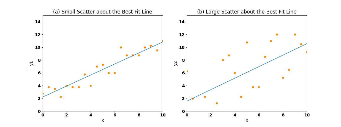
Fig. 12 Scatter plots showing (a) small scatter/spread and (b) large scatter/spread of points about the best fit line.

If the points are closely packed about the regression line, then the fit is considered to be “good”. Quantitatively, the measure of the spread of the points about the best fit line is given by the correlation coefficient, $r$.

Correlation Coefficient

Let’s start to write down the expression for the correlation coefficient. What we aim to do is to come up with an expression that tells us how much of the original variance in $y(t)$ is captured by the fit, $\hat{y}(t)$. We will start by defining the total sum of squares for $y(t)$, $S_{yy}$,

$$S_{yy}=\sum _{i=1}^N(y_i(t)-\bar{y}{)}^2$$

This is essentially the variance of $y(t)$ except that we are not dividing by $N$, just to keep things simple.

Next, let’s write down an expression for the sum of squares for $\widehat{y(t)}$, which represents the variance in the fit between $x(t)$ and $y(t)$ (except again, we are not going to divide by $N$),

$$\begin{array}{r}\begin{array}{rl}{S}_{\hat{y}\hat{y}}& =\sum _{i=1}^N(\widehat{y_i}(t)-\bar{\hat{y}}{)}^2\\ & =\sum _{i=1}^N(\widehat{y_i}(t)-\bar{y}{)}^2\end{array}\end{array}$$

You can prove to yourself that $\bar{\hat{y}}$ = $\bar{y}$.

So, now we have the two parts of the expression that we need. The ratio of $S_{\hat{y}\hat{y}}$ to $S_{yy}$ tells of the fraction of the totoal variance in $y(t)$ explained by the variance of the fit. This ratio is called the coefficient of determination, $r^2$. The coefficient of determination is the correlation coefficient squared!

$$\begin{array}{r}\begin{array}{rl}{r}^2& =\frac{\text{explained variance}}{\text{total variance}}\\ & =\frac{S_{\hat{y}\hat{y}}}{S_{yy}}\\ & \\ & \text{Plugging in the expression for }\hat{y}(t)\text{ and rearranging things, we get ...}\\ & \\ & =\frac{(\overline{x^{\prime }{y}^{\prime }}{)}^2}{\overline{{x^{\prime }}^2}\overline{{y^{\prime }}^2}}\end{array}\end{array}$$

We are not going to worry about all the algebra required to get to the final expression for the coefficient of determination, but if you are interested you can take a look here.

So, the correlation coefficient is the square-root of $r^2$,

$$\begin{array}{r}\begin{array}{rl}r& =\pm \sqrt{r^2}\\ & =\frac{\overline{x^{\prime }{y}^{\prime }}}{{\sigma }_x{\sigma }_y}\end{array}\end{array}$$

To summarize the above:

$r^2$, the coefficient of determination (aka “r-squared”):

• is the fraction of variance explained by the linear least-squares fit between the two variables

• always lies between 0 and 1

r, the correlation coefficient:

• varies between -1 and 1

• indicates the sign of the relationship between the two variables

The table below shows some values of $r$ and $r^2$.

Correlation Coefficient	Coefficient of Determination
0.99	0.98
0.90	0.81
0.70	0.49
0.50	0.25
0.25	0.06

Let’s take a look at how good the fit between ENSO and California precipitation is by calculating the correlation coefficient.

# load packages
import numpy as np
import pickle as pickle
import scipy.stats as st
import matplotlib.pyplot as plt
import matplotlib as mpl
mpl.rc('font',size=16,weight='bold') #set default font size and weight for plots

Let’s load in our ENSO and California precipitation data again.

# ENSO Data:
# unpickle NINO34 (units of degC)
with open('NINO34_NDJF_2021.pickle','rb') as fp: #.pickle files are a python file type
    nino34 = pickle.load(fp,encoding='latin1')

#  Precipitation Data:
#  unpickle CA_PRECIP_DJFM (units of mm/day)
with open('CA_PRECIP_DJFM.pickle','rb') as fp: #.pickle files are a python file type
    precip_djfm = pickle.load(fp,encoding='latin1')

We will take a look at two ways to compute the correlation coefficient, first using np.corrcoeff() and second using stats.pearsonr().

# np.corrcoef computes the correlation matrix, 
# i.e. it computes the correlation between nino34 and itself, precip_djfm and itself and nino34 and precip_djfm

r = np.corrcoef(nino34,precip_djfm)
print(r)

[[1.        0.5020922]
 [0.5020922 1.       ]]

The correlation between ENSO and California precipitation are the correlations on the off-diagonals while the correlations of each variable with itself are identically 1.0 and along the diagonal.

# extract the correlation we want using slicing
r = np.corrcoef(nino34,precip_djfm)[0,1]
print(r)

0.5020922027309632

We can also calculate the correlation coefficient using the following function. This function also provides the p-value for the correlation (we will talk more about computing the statistical significance of correlations in the next section).

# alternative correlation coefficient function including the p-value
pearsons_corrcoef, p_corr = st.pearsonr(nino34,precip_djfm)
print("The correlation = ", pearsons_corrcoef, "with a very small p-value of", p_corr, "i.e., very significant!")

The correlation =  0.5020922027309634 with a very small p-value of 2.6350145043512816e-71 i.e., very significant!

We find that the correlation between ENSO and California precipitation is positive and approximately 0.5. We can express this as the fraction of variance explained by the fit using the r-squared.

# calculate r-squared (aka coefficient of determination)
r2 = r**2
print(r2)

0.25209658004323066

So, the fraction of variance in California precipitation explained by ENSO is about 25%. That’s actually a fair bit considering all the meteorological phenomena that can affect precipitation.